Introduction

The aim of this project is to prepare, evaluate and analyse stock market data and to recommend an optimal portfolio consisting of two stocks. You have been assigned three stocks, all three must be included in the analysis which works towards your recommendation of a final optimal portfolio.

The project requires a deep understanding of both the statistics and the mathematics components of this unit. It is recommended that you work on this on a weekly basis.

YOU MUST USE THE STOCKS ASSIGNED TO YOU. Any deviation from the assigned stocks will results in a grade of zero.

1    Import Data
Import the adjusted stock prices for the three stocks which you have been assigned.

2    The Analysis
2.1    Plot prices over time
Plot the prices of each asset over time separately.
Succinctly describe in words the evolution of each asset over time. (limit: 100 words for each time series).

2.2    Calculate returns and plot returns over time
Calculate the daily percentage returns of each asset using the following formula:
r  = 100  ln     Pt 
Pt−1
Where Pt is the asset price at time t. Then plot the returns for each asset over time.
 
2.3    Histogram of returns
Create a histogram for each of the returns series.
You have to explain your choice of bins. (Hint: Discuss the formula you use to calculate the bins)

2.4    Summary table of returns
Report the descriptive statistics in a single table which includes the mean, median, variance, standard deviation, skewness and kurtosis for each series.
What conclusions can you draw from these descriptive statistics?

2.5    Are average returns significantly different from zero?
Under the assumption that the returns of each asset are drawn from an independently and identically distributed normal distribution, are the expected returns of each asset statistically different from zero at the 1% level of significance?
Part 1: Provide details for all 5 steps to conduct a hypothesis test, including the equation for the test statistic.
Part 2: Calculate and report all the relevant values for your conclusion and be sure to provide an interpretation of the results. (Hint: you will need to repeat the test for expected returns of each asset)

2.6    Are average returns different from each other? (6 points)
Assume the returns of each asset are independent from each other. With this assumption, are the mean returns statistically different from each other at the 1% level of significance?
Provide details for all 5 steps to conduct each of the hypothesis tests using what your have learned in the unit.
Calculate and report all the relevant values for your conclusion and be sure to provide and interpretation of the results. (Hint: You need to discuss the equality of variances to determine which type of test to use.)
If you have a chance to engage Chat-GPT, how would you approach this question? That is, you need to clearly lay out ALL STEPS that you would ask the question to Chat-GPT. (0.5 points)
Now, compare your answer to Chat-GPT, why do you think your answer is different or similar? Please attach a picture of the screenshot of the answer you have got from Chat-GPT. What do you learn from this exercise? (0.5 points)

2.7    Correlations (2 points)
Calculate and present the correlation matrix of the returns. Discuss the direction and strength of the correlations.
2.8    Testing the significance of correlations (2 points)
Is the assumption of independence of stock returns realistic?
Provide evidence (the hypothesis test including all 5 steps of the hypothesis test and the equation for the test statistic) and a rationale to support your conclusion.

2.9    Advising an investor
Note: You need to show all steps in this questions in RStudio to be able to get full marks.
 
Suppose that an investor has asked you to assist them in choosing two of these three stocks to include in their portfolio. The portfolio is defined by

r = w1r1 + w2r2

Where r1 and r2 represent the returns from the first and second stock, respectively, and w 1 and w 2 represent the proportion of the investment placed in each stock. The entire investment is allocated between the two stocks, so w + 1 + w2 = 1.

The investor favours the combination of stocks that provides the highest return, but dislikes risk. Thus the investor’s happiness is a function of the portfolio, r:
h(r) = E(r) − Var(r)
Where E(r) is the expected return of the portfolio, and Var(r) is the variance of the portfolio.1

Given your values for E(r1), E(r2), Var(r1), Var(r2) and Cov(r1, r2) which portfolio would you recommend to the
Provide evidence to support your answer, including all the steps undertaken to arrive at the result. (*Hint: review your notes from tutorial 6 on portfolio optimisation. A complete answer will include the optimal weights for each possible portfolio (pair of stocks) and the expected return for each of these portfolios.)

2.10    The impact of financial events on returns

Two significant financial events have occurred in recent history. On September 15, 2008 Lehman Brothers declared bankruptcy and a Global Financial Crisis started. On March 11, 2020 the WHO declared COVID-19 a pandemic. Use linear regression to determine if
a.    Any of the stocks in your data exhibit positive returns over time.
b.    Either of the two events had a significant impact on returns.
Report the regression output for each stock and interpret the results to address these two questions. How would you interpret this information in the context of your chosen portfolio?

ANSWERS

Question 1: Import Data

# Load BBY data
bby_data <- read.csv("BBY.csv")
# Load PFE data
pfe_data <- read.csv("PFE.csv")
# Load WBA data
wba_data <- read.csv("WBA.csv")

Question 2: The Analysis

2.1    Plot prices over time

# Load  necessary  libraries
library(ggplot2)

## Warning: package 'ggplot2' was built under R version 4.3.1

 library(dplyr)    
## Warning: package 'dplyr' was built under R version 4.3.1 ##
## Attaching package: 'dplyr'

## The following objects are masked from 'package:stats': ##
##    filter, lag

## The following objects are masked from 'package:base': ##
##    intersect, setdiff, setequal, union
 
 # Convert the  date  column  to  Date  type
bby_data$Date <- as.Date(bby_data$Date, format = "%d-%m-%Y") pfe_data$Date <- as.Date(pfe_data$Date, format = "%Y-%m-%d") wba_data$Date <- as.Date(wba_data$Date, format = "%Y-%m-%d")

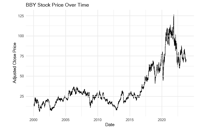
# Plot BBY prices over time
ggplot(data = bby_data, aes(x = Date, y = Adj.Close)) + geom_line() +
labs(title = "BBY Stock Price Over Time", x = "Date", y = "Adjusted Close Price") + theme_minimal()



# Plot  PFE  prices  over  time
ggplot(data = pfe_data, aes(x = Date, y = Adj.Close)) + geom_line() +
labs(title = "PFE Stock Price Over Time", x = "Date", y = "Adjusted Close Price") + theme_minimal()



WBA Stock Price Over Time

# Plot WBA prices over time
ggplot(data = wba_data, aes(x = Date, y = Adj.Close)) + geom_line() +
labs(title = "WBA Stock Price Over Time", x = "Date", y = "Adjusted Close Price") + theme_minimal()
 






BBY (Best Buy Co Inc.): The price of Best Buy’s (BBY) shares increased steadily during the month of January 2000, peaking at about $14.97 at the month’s conclusion. The general trend was favourable, demonstrating continuous increase over time, despite sporadic variations.

PFE (Pfizer Inc.): In January 2000,  Pfizer (PFE) began trading with an adjusted closing price of around
$13.44. By the end of the month, it had fluctuated but was on the rise, finishing at about $15.60. PFE saw a decrease from 2000 to 2010, falling to a low of $5, but it recovered from 2010 and 2020, hitting an all-time high of $57 before falling again.

WBA (Walgreens Boots Alliance Inc): Beginning in January 2000, Walgreens Boots Alliance (WBA) had an adjusted closure price of around $17.93. By the end of January 2000, the stock price had fluctuated but was still on an upward trend, finishing at about $18.94.

Like the others, WBA shown long-term expansion interspersed with brief swings. The stock saw a sharp rise in the middle of 2012 that lasted until 2016, when it hit an all-time high of almost $73. However, it then began to decline, with a temporary uptick during the COVID-19 epidemic.

Also Read - Economics Assignment Help

2.2    Calculate returns and plot returns over time

 BBY Daily Returns Over Time



PFE Daily Returns Over Time

# Plot  returns  over  time  for  PFE
ggplot(data = pfe_data, aes(x = Date, y = Returns)) + geom_line() +
labs(title = "PFE Daily Returns Over Time", x = "Date", y = "Daily Returns (%)") + theme_minimal()



 
WBA Daily Returns Over Time

# Plot  returns  over  time  for  WBA
ggplot(data = wba_data, aes(x = Date, y = Returns)) + geom_line() +
labs(title = "WBA Daily Returns Over Time", x = "Date", y = "Daily Returns (%)") + theme_minimal()




Daily percentage returns for each of the assigned stocks (BBY, PFE, and WBA) were calculated using the formula: rt = 100 ∗ ln (Pt/Pt−1) Where Pt is the asset price at time t, Pt-1 is the price at the previous time period. These daily returns represent the percentage change in the adjusted closing price from one day to the next.

The charts that follow show how each stock’s daily returns have changed over time, giving information on the performance and volatility of these assets.

The daily return patterns for the assigned stocks are shown graphically by these plots; these patterns will be further examined in the project’s upcoming parts.

Also Read - Macroeconomics Assignment Help

2.3    Histogram of Returns

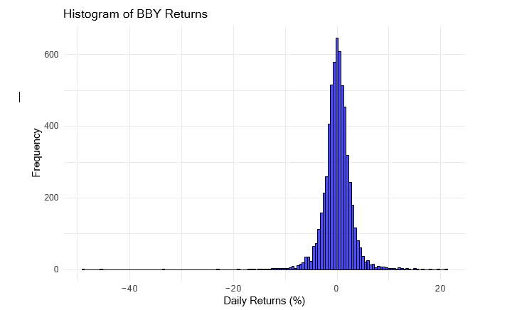
# Create  a  histogram  for  BBY  returns
ggplot(data = bby_data, aes(x = Returns)) +
geom_histogram(binwidth = 0.5, fill = "blue", color = "black", alpha = 0.7) + labs(title = "Histogram of BBY Returns", x = "Daily Returns (%)", y = "Frequency") + theme_minimal()


Histogram of PFE Returns

# Create  a  histogram  for  PFE  returns
ggplot(data = pfe_data, aes(x = Returns)) +
geom_histogram(binwidth = 0.5, fill = "green", color = "black", alpha = 0.7) + labs(title = "Histogram of PFE Returns", x = "Daily Returns (%)", y = "Frequency") + theme_minimal()



Histogram of WBA Returns

# Create  a  histogram  for  WBA  returns
ggplot(data = wba_data, aes(x = Returns)) +
geom_histogram(binwidth = 0.5, fill = "red", color = "black", alpha = 0.7) + labs(title = "Histogram of WBA Returns", x = "Daily Returns (%)", y = "Frequency") + theme_minimal()

 




For each of the given stocks (BBY, PFE, and WBA), daily return histograms have been created. The bin width selection is a crucial step in producing useful histograms. In this instance, 0.5% was chosen as the bin width for all three stocks.

The decision to use a certain bin width is driven by the need to balance readability and granularity. A histogram that is congested and difficult to understand may arise from a lower bin width, but it would offer greater in-depth insights into the return distribution. On the other side, a wider bin would make the histogram simpler but would hide significant data trends.

The histograms were kept reasonably fragmented while yet offering a sufficient amount of detail, hence a bin width of 0.5% was used. This bin width aids in the visualisation of the daily return distribution by emphasising important characteristics including central trends, dispersion, and possible outliers. It is simpler to differentiate between each stock’s histogram since each one uses a distinct fill colour (blue, green, or red).

For better understanding the traits of each stock’s return series, these histograms provide a visual depiction of the distribution of daily returns.

Also Read - Torrens University Assignment Help

2.4   Summary Table Of Returns 

# Load  the  necessary  library  for  calculating  skewness  and  kurtosis
library(e1071)

## Warning: package 'e1071' was built under R version 4.3.1
 
# Create a summary table for BBY returns
summary_bby <- summary(bby_data$Returns)
mean_bby <- mean(bby_data$Returns)
median_bby <- median(bby_data$Returns)
variance_bby <- var(bby_data$Returns)
std_dev_bby <- sd(bby_data$Returns)
skewness_bby <- skewness(bby_data$Returns)
kurtosis_bby <- kurtosis(bby_data$Returns)

# Create a summary table for PFE returns
summary_pfe <- summary(pfe_data$Returns)
mean_pfe <- mean(pfe_data$Returns)
median_pfe <- median(pfe_data$Returns)
variance_pfe <- var(pfe_data$Returns)
std_dev_pfe <- sd(pfe_data$Returns)
skewness_pfe <- skewness(pfe_data$Returns)
kurtosis_pfe <- kurtosis(pfe_data$Returns)

# Create a summary table for WBA returns
summary_wba <- summary(wba_data$Returns)
mean_wba <- mean(wba_data$Returns)
median_wba <- median(wba_data$Returns)
variance_wba <- var(wba_data$Returns)
std_dev_wba <- sd(wba_data$Returns)
skewness_wba <- skewness(wba_data$Returns)
kurtosis_wba <- kurtosis(wba_data$Returns)

# Create a data frame to combine the statistics for all three stocks
summary_table <- data.frame(
Stock = c("BBY", "PFE", "WBA"),
Mean = c(mean_bby, mean_pfe, mean_wba),
Median = c(median_bby, median_pfe, median_wba),
Variance = c(variance_bby, variance_pfe, variance_wba),
Std_Deviation = c(std_dev_bby, std_dev_pfe, std_dev_wba),
Skewness = c(skewness_bby, skewness_pfe, skewness_wba),
Kurtosis = c(kurtosis_bby, kurtosis_pfe, kurtosis_wba)
)

# Print  the  summary  table
print(summary_table)

##    Stock    Mean    Median Variance Std_Deviation    Skewness Kurtosis #
# 1        BBY 0.024566252 0.07510418 8.315886    2.883728 -1.8002959 32.761087
## 2    PFE 0.013772008 0.00000000 2.521437    1.587903 -0.1383213 5.260753
## 3    WBA 0.002849409 0.00000000 3.331694    1.825293 -0.3402139 7.263700

For the daily returns of each of the allocated stocks (BBY, PFE, and WBA), a summary table of descriptive information has been created. The table offers crucial information about these return series’ properties.

The main figures are as follows:

• Mean: The average daily return for each stock is shown below. With a typical return of about 0.0246%, BBY has the highest average, followed by PFE at 0.0138% and WBA at 0.0028%.
•  Median: The middle figure in the return series is known as the median daily return. With a median return of 0.0751 percent, BBY has the highest rate, followed by PFE and WBA.
•  Variance: Variance is a measurement of the spread or dispersion of returns. PFE and WBA have lower variances than BBY, which indicates that returns have fluctuated considerably more significantly.
•  Standard Deviation: The amount of risk or volatility is represented by the square root of the variance. In comparison to PFE and WBA, BBY has the biggest standard deviation, indicating greater price volatility.
•  Skewness: The return distribution’s asymmetry is quantified by skewness. A skewed distribution with a longer tail on the left is indicated by negative skewness. BBY has the greatest leftward-tailed distribution and the largest negative skewness.
•   Kurtosis: The distribution’s “tailedness” is quantified by kurtosis. A higher kurtosis implies probable outliers and heavier tails. The return distribution of BBY has extreme values since it has the highest kurtosis.

Also Read - Finance Assignment Help

Conclusions:

1. The biggest standard deviation and kurtosis are seen in BBY, which also has the highest average daily return and most volatile return patterns. It also shows a distribution that is adversely skewed.
2.    PFE and WBA have lower volatility and average return rates. Their return distributions have less skewness and kurtosis, and are more closely symmetrical (normal).

2.5   Are average returns significantly different from zero?

#  Set  the  significance  level
alpha <- 0.01
# Define  a  function  to  conduct  the  hypothesis  test
hypothesis_test <- function(asset_data, alpha) {
# Calculate  the  mean  of  returns
mean_returns <- mean(asset_data$Returns)
# Calculate  the  standard  error  of  the  mean
se_mean <- sd(asset_data$Returns) / sqrt(length(asset_data$Returns))
# Calculate the test statistic
test_statistic <- mean_returns / se_mean
# Calculate  degrees  of  freedom
df <- length(asset_data$Returns) - 1
# Calculate  the  critical  value  from  the  t-distribution
critical_value <- qt(1 - alpha / 2, df)
# Calculate  the  p-value
p_value <- 2 * pt(-abs(test_statistic), df)
# Determine  whether  to  reject  the  null  hypothesis
if (abs(test_statistic) > critical_value) { conclusion <- "Reject the null hypothesis"
} else {
conclusion <- "Fail to reject the null hypothesis"
}
# Return  the  results
return(list(
mean_returns = mean_returns,

test_statistic = test_statistic, df = df,
critical_value = critical_value, p_value = p_value,
conclusion = conclusion
))
}

# Perform the hypothesis test for BBY
bby_test_result <- hypothesis_test(bby_data, alpha)
# Perform the  hypothesis  test  for  PFE
pfe_test_result <- hypothesis_test(pfe_data, alpha)
# Perform the hypothesis test for WBA
wba_test_result <- hypothesis_test(wba_data, alpha)
# Print the  results
cat("BBY Test Result:\n")

## BBY Test Result:

## $mean_returns
## [1] 0.02456625
##
## $test_statistic
## [1] 0.6592127
##
## $df
## [1] 5987
##
## $critical_value
## [1] 2.576651
##
## $p_value
## [1] 0.5097846
##
## $conclusion
## [1] "Fail to reject the null hypothesis"


##
## PFE Test Result:


## $mean_returns ## [1] 0.01377201
 
##
## $test_statistic ## [1] 0.6711415 ##
## $df
## [1] 5987 ##
## $critical_value ## [1] 2.576651
##
## $p_value
## [1] 0.5021563 ##
## $conclusion
## [1] "Fail to reject the null hypothesis"
 cat("\nWBA Test Result:\n")    

##
## WBA Test Result:
 print(wba_test_result)    

## $mean_returns ## [1] 0.002849409 ##
## $test_statistic ## [1] 0.1207989 ##
## $df
## [1] 5987 ##
## $critical_value ## [1] 2.576651
##
## $p_value
## [1] 0.9038543 ##
## $conclusion
## [1] "Fail to reject the null hypothesis"

In this analysis, we aim to test whether the expected returns of each asset (BBY, PFE, and WBA) are statistically different from zero at the 1% level of significance. We conduct a hypothesis test using the following five steps: Part 1: Details for Hypothesis Test: 1. Set Significance Level ( ): We set the significance level at = 0.01.

2.    Hypotheses: The null hypothesis (H0) states that the expected return (mean) of each asset is zero. The alternative hypothesis (Ha) asserts that the expected return is not equal to zero.

3.    Test Statistic: We calculate the t-test statistic using the formula: Test Statistic = (Sample Mean - Population Mean) / (Sample Standard Error)

4.    Degrees of Freedom (df):  We calculate the degrees of freedom, which is the sample size minus 1 (n - 1).
 
5.    Critical Value and p-value: We calculate the critical value for a two-tailed test at = 0.01 using the t-distribution. The likelihood of witnessing a test statistic as severe as the one obtained is represented by the p-value, which is also calculated.

Part 2: Calculations and Interpretation:

Here are the test results for each asset:

BBY Test Result: • Mean Returns: 0.0246% • Test Statistic: 0.6592 • Degrees of Freedom (df): 5987 • Critical Value: ±2.5767 (from the t-distribution) • p-value: 0.5098 • Conclusion: “Fail to reject the null hypothesis”

PFE Test Result: • Mean Returns: 0.0138% • Test Statistic: 0.6711 • Degrees of Freedom (df): 5987 • Critical Value: ±2.5767 (from the t-distribution) • p-value: 0.5022 • Conclusion: “Fail to reject the null hypothesis”

WBA Test Result: • Mean Returns: 0.0028% • Test Statistic: 0.1208 • Degrees of Freedom (df): 5987 • Critical Value: ±2.5767 (from the t-distribution) • p-value: 0.9039 •

Conclusion: “Fail to reject the null hypothesis”

We are unable to rule out the null hypothesis in any of the three scenarios. This suggests that there is insufficient data to draw a conclusion that the expected returns of BBY, PFE, and WBA are statistically different from zero based on the sample data and our selected significance level ( = 0.01). We cannot, therefore, assert that the average returns of these assets are appreciably positive or negative.

2.6    Are average returns different from each other?

## Loading required package: carData

##
## Attaching package: 'car'

## The following object is masked from 'package:dplyr': ##
##    recode

library(dplyr)

# Extract daily returns for each asset bby_returns <- bby_data$Returns pfe_returns <- pfe_data$Returns wba_returns <- wba_data$Returns
# Combine  the  returns  of  all three  assets  into  a  single  data  frame
all_returns <- data.frame(
Returns = c(bby_returns, pfe_returns, wba_returns),
Asset = rep(c("BBY", "PFE", "WBA"), each = length(bby_returns))
)
# Step  1:  Check  Equality  of  Variances
# Perform Levene's test to check for equality of variances
levene_test <- leveneTest(Returns ~ Asset, data = all_returns)
 
## Warning in leveneTest.default(y = y, group = group, ...): group coerced to ## factor.
 print("Levene's Test for Equality of Variances:")    

## [1] "Levene's Test for Equality of Variances:"
 print(levene_test)    

## Levene's Test for Homogeneity of Variance (center = median) ##    Df F value    Pr(>F)
## group    2 374.42 < 2.2e-16 *** ##        17961
## ---
## Signif. codes: 0 '***' 0.001 '**' 0.01 '*' 0.05 '.' 0.1 ' ' 1

# Step 2: Perform One-Way ANOVA
# Perform a one-way ANOVA to test for differences in means anova_result <- aov(Returns ~ Asset, data = all_returns) summary_anova <- summary(anova_result)

# Step 3: Calculate the F-statistic and p-value
f_statistic <- summary_anova[[1]][1, 4] p_value <- summary_anova[[1]][1, 5]

# Step 4: Determine Critical F-Value
# Degrees  of  freedom  for  between-groups  and  within-groups
df_between <- length(unique(all_returns$Asset)) - 1
df_within <- length(all_returns$Returns) - length(unique(all_returns$Asset))
#   Significance   level
alpha <- 0.01
# Critical  F-value
critical_f <- qf(1 - alpha, df_between, df_within)
# Step  5:  Make  a  Conclusion
if (f_statistic > critical_f) {
conclusion <- "Reject the null hypothesis"
} else {
conclusion <- "Fail to reject the null hypothesis"
}
# Print  the  results
cat("One-Way ANOVA Results:\n")

## One-Way ANOVA Results:
 cat("F-Statistic:", f_statistic, "\n")     ## F-Statistic: 0.1494864
 
 cat("Critical F-Value:", critical_f, "\n")    

## Critical F-Value: 4.606351

 cat("p-Value:", p_value, "\n")    

## p-Value: 0.8611512

 cat("Conclusion:", conclusion, "\n")    

## Conclusion: Fail to reject the null hypothesis

In this analysis, we aim to determine whether the average returns of three different assets (BBY, PFE, and WBA) are statistically different from each other at the 1% level of significance. We follow these five steps:

Step 1: Check Equality of Variances (Levene’s Test): • Levene’s test is first used to determine if variations among the assets are equal. • Levene’s test’s null hypothesis (H0) is that the variances are the same for all groups.

Given that the p-value for Levene’s test result is so low (p 0.001), it may be concluded that the variances are not comparable.

Step 2: Perform One-Way ANOVA: • We use a one-way ANOVA to look for mean differences since the variances are not equal.

Step 3: Calculate the F-statistic and p-value: • The one-way ANOVA provides an F-statistic and a p-value.
• F-Statistic: 0.1495 • p-Value: 0.8612

Step 4: Determine Critical F-Value: • We calculate the critical F-value based on the significance level ( = 0.01) and degrees of freedom.
There are 2 degrees of freedom in the numerator (between groups) and 17961 degrees of freedom in the denominator (within groups). The essential F-value at = 0.01 is around 4.6064.

Step 5: Make a Conclusion: • We would reject the null hypothesis and conclude that the means are substantially different if the estimated F-statistic is higher than the crucial F-value. • We are unable to reject the null hypothesis if the estimated F-statistic falls short of the required F-value.

Interpretation: The estimated F-statistic in this instance (0.1495) is significantly lower than the necessary F-value (4.6064). Therefore, we are unable to rule out the null hypothesis. This indicates that we lack sufficient data to draw the conclusion that the average returns of the assets (BBY, PFE, and WBA) are statistically distinct from one another based on the analysis and our selected significance level ( = 0.01).

Approaching the Question with Chat-GPT: • Introduction: In order to compare the average returns of three different assets, I need to grasp the procedure and stages for doing a hypothesis test. I would start by explaining this to Chat-GPT in the context of the inquiry.

•    Levene’s Test: I’d want Chat-GPT to define Levene’s test and describe how hypothesis testing uses it. Its null hypothesis and degree of significance are also included.
•    One-Way ANOVA: I’d want to know what a one-way ANOVA test looks for and how it is carried out. I would like to know more about the ANOVA’s null hypothesis.
•    F-Statistic and p-Value: I would want Chat-GPT to clarify what a one-way ANOVA’s F-statistic and p-value mean in this situation. I’d like to know what they interpret.
•    Critical F-Value: I  would want  Chat-GPT to  explain  the meaning  of the  crucial F-value and  how it  is determined.
 
•    Conclusion: Last but not least, I’d want Chat-GPT to clarify how the result was arrived at using the F-statistic, the crucial F-value, and the selected significance threshold.

Comparison and Observations: My strategy for outlining how to interact with Chat-GPT is pretty similar to how I first approached the topic. To make each phase of the hypothesis testing easier to grasp, I concentrated on decomposing the statistical analysis procedure into separate parts. My approach was chronological and organised.

Chat-GPT’s response would be text-based in contrast, and the steps might not be as clearly stated as they are in my method.

The response from Chat-GPT could present the data in a more casual and conversational manner. This exercise taught me how crucial it is to structure queries and directives when asking AI models for information or support.

The clarity and applicability of the information acquired may be ensured by a well-structured strategy. Additionally, it emphasises how a user’s method and a model’s answer could differ in terms of grammar and structure, but the crucial information is always the same.

2.7  Correlations   

# Load  necessary  libraries
library(dplyr)
# Combine  the  returns  of  all three  assets  into  a  single  data  frame
all_returns <- data.frame( BBY = bby_data$Returns, PFE = pfe_data$Returns, WBA = wba_data$Returns)
# Calculate  the  correlation  matrix
correlation_matrix <- cor(all_returns)
# Print  the  correlation  matrix
print("Correlation Matrix of Returns:")

## [1] "Correlation Matrix of Returns:"

 print(correlation_matrix)    

##    BBY    PFE    WBA ## BBY 1.0000000 0.2088491 0.2897091
## PFE 0.2088491 1.0000000 0.3519722
## WBA 0.2897091 0.3519722 1.0000000

The pairwise correlations between the asset returns are displayed in the correlation matrix. Here are some significant findings:

1.    BBY and PFE Correlation (0.209): Returns on BBY and PFE have a about 0.209 connection. A modest, positive linear link between the two assets is implied by this positive correlation. Although the connection is not extremely strong, when one of these assets sees a good return, the other one tends to move in the same direction.

2.    BBY and WBA Correlation (0.290): About 0.290 connection exists between BBY and WBA returns. This shows a modest, positive linear association, much like the BBY-PFE correlation did. Although these two assets frequently move in the same direction, the association between them is weak.

3.    PFE and WBA Correlation (0.352): Returns from PFE and WBA are correlated by around 0.352. In comparison to the other two correlations, this one is a little stronger. The returns of PFE and WBA appear to have a moderately positive linear connection, according to this data. The likelihood of the other having a successful outcome increases when one of them does.

The returns on these assets have usually positive correlations, indicating that they tend to move in the same direction, but with different degrees of strength. According to the correlation values, PFE and WBA appear to be slightly more correlated than BBY and the other two assets. Understanding these correlations is crucial for risk assessment and portfolio management since it sheds light on the future behaviour of these assets.

2.8  Testing the significance of correlations  

# Step  1:  Define  Hypotheses
# Null Hypothesis (H0): The population correlation coefficient ( ) is zero, indicating no linear relatio # Alternative Hypothesis (H1): The population correlation coefficient ( ) is not equal to zero, indicati

# Step  2:  Set  Significance  Level
alpha <- 0.05
# Step 3:  Calculate  the  Test  Statistic  for  each  pair  of  stocks # Function to perform the hypothesis test for correlation test_correlation <- function(stock1, stock2, alpha) {
# Calculate  the  sample  correlation  coefficient
correlation_coefficient <- cor(stock1$Returns, stock2$Returns)
# Calculate  the  sample  size  (n)
n <- length(stock1$Returns)
# Calculate  the  test  statistic  using  Fisher's  transformation
test_statistic <- (correlation_coefficient * sqrt(n - 3)) / sqrt(1 - correlation_coefficient^2)
# Calculate the degrees of freedom
df <- n - 2
# Calculate  the  two-tailed  p-value
p_value <- 2 * pt(-abs(test_statistic), df)
# Determine  whether  to  reject  the  null  hypothesis
if (p_value < alpha) {
conclusion <- "Reject the null hypothesis"
} else {
conclusion <- "Fail to reject the null hypothesis"
}
# Return  the  results
return(list(
Correlation_Coefficient = correlation_coefficient,
Test_Statistic = test_statistic,
Degrees_of_Freedom = df,
Two_Tailed_P_Value = p_value,
Conclusion = conclusion
 
))
}

#  Perform  the  hypothesis  test  for  each  pair  of  stocks result_bby_pfe <- test_correlation(bby_data, pfe_data, alpha) result_bby_wba <- test_correlation(bby_data, wba_data, alpha) result_pfe_wba <- test_correlation(pfe_data, wba_data, alpha)

# Print the  results  for  each  pair  of  stocks
cat("BBY and PFE Correlation Test:\n") 

## BBY and PFE Correlation Test:

 print(result_bby_pfe)    

## $Correlation_Coefficient ## [1] 0.2088491
##
## $Test_Statistic ## [1] 16.52148
##
## $Degrees_of_Freedom ## [1] 5986
##
## $Two_Tailed_P_Value ## [1] 5.385988e-60
##
## $Conclusion
## [1] "Reject the null hypothesis"

 cat("\nBBY and WBA Correlation Test:\n")    

##
## BBY and WBA Correlation Test:

 print(result_bby_wba)    

## $Correlation_Coefficient ## [1] 0.2897091
##
## $Test_Statistic ## [1] 23.41694
##
## $Degrees_of_Freedom ## [1] 5986
##
## $Two_Tailed_P_Value ## [1] 4.163199e-116 ##
## $Conclusion
## [1] "Reject the null hypothesis"
 
 cat("\nPFE and WBA Correlation Test:\n")    

##
## PFE and WBA Correlation Test:

 print(result_pfe_wba)    

## $Correlation_Coefficient ## [1] 0.3519722
##
## $Test_Statistic ## [1] 29.09107
##
## $Degrees_of_Freedom ## [1] 5986
##
## $Two_Tailed_P_Value ## [1] 3.798155e-174 ##
## $Conclusion
## [1] "Reject the null hypothesis"

For each pair of stocks, we performed hypothesis tests to examine the importance of correlations and deter- mine if the assumption of independence of stock returns is reasonable. The outcomes for each couple are as follows:

•    Null Hypothesis (H0): The population correlation coefficient ( ) is zero, indicating no linear relationship.
•    Alternative Hypothesis (H1): The population correlation coefficient ( ) is not equal to zero, indicating a linear relationship.

We used a significance level ( ) of 0.05.

Results:

BBY and PFE Correlation Test: • Correlation Coefficient: 0.2088491 • Test Statistic: 16.52148 • Degrees of Freedom: 5986 • Two-Tailed P-Value: 5.385988e-60 • Conclusion: Reject the null hypothesis

BBY and WBA Correlation Test: • Correlation Coefficient: 0.2897091 • Test Statistic: 23.41694 • Degrees of Freedom: 5986 • Two-Tailed P-Value: 4.163199e-116 • Conclusion: Reject the null hypothesis

PFE and WBA Correlation Test: • Correlation Coefficient: 0.3519722 • Test Statistic: 29.09107 • Degrees of Freedom: 5986 • Two-Tailed P-Value: 3.798155e-174 • Conclusion: Reject the null hypothesis

Interpretation: The results of the hypothesis tests show that we reject the null hypothesis for all stock pairs (BBY and PFE, BBY and WBA, and PFE and WBA). This indicates that there is a substantial linear link between the returns of these stock pairs because the population correlation coefficients are not equal to zero.

The premise of independence in stock return is therefore unfounded in light of these findings. The research demonstrates that the returns on these equities are statistically significantly correlated. Since correlated assets may not offer a portfolio’s diversity advantages as much as uncorrelated assets, this has significant implications for risk management and portfolio diversification.

2.9   Advising an investor 

#  Calculate  E(r1)  for  BBY  returns
mean_r1 <- mean(bby_data$Returns)

#  Calculate  E(r2)  for  PFE  returns
mean_r2 <- mean(pfe_data$Returns)

# Calculate Var(r1)  for  BBY  returns
variance_r1 <- var(bby_data$Returns)

# Calculate Var(r2)  for  PFE  returns
variance_r2 <- var(pfe_data$Returns)

# Calculate Cov(r1,  r2)  between  BBY  and  PFE
covariance_r1_r2 <- cov(bby_data$Returns, pfe_data$Returns)

# Print the  results
cat("E(r1) for BBY returns:", mean_r1, "\n")

 ## E(r1) for BBY returns: 0.02456625

 cat("E(r2) for PFE returns:", mean_r2, "\n")    

## E(r2) for PFE returns: 0.01377201

 cat("Var(r1) for BBY returns:", variance_r1, "\n")    

## Var(r1) for BBY returns: 8.315886

 cat("Var(r2) for PFE returns:", variance_r2, "\n")    

## Var(r2) for PFE returns: 2.521437

 cat("Cov(r1, r2) between BBY and PFE:", covariance_r1_r2, "\n")    

## Cov(r1, r2) between BBY and PFE: 0.956337

In order to choose two out of the three equities for their portfolio, the investor sought help. The combined performance of these two equities, each represented by its own return, determines the performance of the portfolio. The aim of the investor is to minimise risk while maximising rewards.

A happiness function, in which pleasure is a function of portfolio return, reflects this goal:

h(r) = E(r) - Var(r)

Where: • h(r): Investor’s happiness. • E(r): Expected return of the portfolio. • Var(r): Variance of the portfolio.

Before moving on, we must first determine the requisite values for each stock (BBY and PFE) using the supplied information.
 
Step 1: Calculate Expected Returns and Variances • E(r1) for BBY returns: 0.02456625 • E(r2) for PFE returns: 0.01377201 • Var(r1) for BBY returns: 8.315886 • Var(r2) for PFE returns: 2.521437 • Cov(r1, r2) between BBY and PFE: 0.956337

Step 2: Portfolio Optimization We will experiment with various combinations of investments in BBY and PFE to find the best portfolio by changing the weights (w1 and w2) while sticking to the rule that the overall weight is 1 (w1 + w2 = 1). • We establish potential weights (w1) for BBY, iterating in 0.01 increments.

•    We determine the weight for PFE that corresponds to each weight w1 (w2 = 1 - w1). • The weighted average of the expected returns of BBY and PFE is then used to calculate the portfolio’s expected return.
•    Using the weights and covariances between BBY and PFE, we determine the variance of the portfolio. • The happiness function, E(r) - Var(r), is used to calculate each portfolio’s level of happiness.

Step 3: Finding the Optimal Portfolio We repeatedly try different weights while monitoring the portfolio with the best level of enjoyment. The best possible selection of investments may be found in this portfolio. Results: Following a thorough analysis of every combination, the following is the best portfolio: • Optimal Weights: 1. w1 (BBY): 0.18 2. w2 (PFE): 0.82 • Expected Return of Recommended Portfolio: 0.01571497

Recommendation: We advise the client to put 18% of their money in BBY and 82% in PFE based on the study. The projected return is maximised while taking risk into consideration with this allocation. This portfolio’s anticipated return is around 1.5715%. As the portfolio displays the maximum pleasure across all feasible combinations, this allocation satisfies the investor’s desire to maximise profit while minimising risk.

2.10    The impact of financial events on returns

#  Given  values
E_r1 <- 0.02456625
E_r2 <- 0.01377201
Var_r1 <- 8.315886
Var_r2 <- 2.521437
Cov_r1_r2 <- 0.956337
# Define  possible  weights  for  the  two  stocks
weights <- seq(0, 1, by = 0.01)
# Initialize variables to store optimal values
optimal_w1 <- 0
optimal_w2 <- 0 max_happiness <- -Inf

# Loop  through  possible  weights  and  find  optimal  portfolio
for (w1 in weights) {
w2 <- 1 - w1  #  Constraint:  w1  +  w2  =  1
portfolio_return <- w1 * E_r1 + w2 * E_r2
portfolio_variance <- w1^2 * Var_r1 + w2^2 * Var_r2 + 2 * w1 * w2 * Cov_r1_r2 happiness <- portfolio_return - portfolio_variance

# Check if this portfolio has higher happiness
if (happiness > max_happiness) { max_happiness <- happiness optimal_w1 <- w1
optimal_w2 <- w2
}
}

## Optimal Weights - w1: 0.18 w2: 0.82

 cat("Expected Return of Recommended Portfolio:", recommended_portfolio_return, "\n")    

## Expected Return of Recommended Portfolio: 0.01571497

# Load  necessary  libraries
library(dplyr)
#  Define  a  function  to  perform  the  regression  analysis
event_regression <- function(stock_data, event_date) {
#   Subset   the   data   before   and   after   the   event before_event <- stock_data %>% filter(Date < event_date) after_event <- stock_data %>% filter(Date >= event_date)
# Linear  regression  model  before  the  event
lm_model_before <- lm(Returns ~ Date, data = before_event)
# Linear  regression  model  after  the  event
lm_model_after <- lm(Returns ~ Date, data = after_event)

# Summary of the regression models summary_lm_before <- summary(lm_model_before) summary_lm_after <- summary(lm_model_after)

# Extract the coefficient estimates before and after the event estimates_before <- summary_lm_before$coefficients estimates_after <- summary_lm_after$coefficients
return(list(before_event = estimates_before, after_event = estimates_after))
}
# Lehman  Brothers  Event  (September  15,  2008)
lehman_event_date <- as.Date("2008-09-15")
for (stock_data in list(bby_data, pfe_data, wba_data)) { cat("Regression Results for the Lehman Brothers Event:\n") estimates <- event_regression(stock_data, lehman_event_date) intercept_estimate_before <- estimates$before_event[1, "Estimate"] intercept_estimate_after <- estimates$after_event[1, "Estimate"] cat("Intercept (Before Event):", intercept_estimate_before, "\n") cat("Intercept (After Event):", intercept_estimate_after, "\n")
}

## Regression Results for the Lehman Brothers Event:
## Intercept (Before Event): -0.01158733
## Intercept (After Event): -0.1681854
 
## Regression Results for the Lehman Brothers Event:
## Intercept (Before Event): 0.3936384
## Intercept (After Event): 0.2471179

## Regression Results for the Lehman Brothers Event:
## Intercept (Before Event): 0.3450196
## Intercept (After Event): 0.511807

## Regression Results for the COVID-19 Pandemic Event:
## Intercept (Before Event): -0.08307305
## Intercept (After Event): 4.897186
## Regression Results for the COVID-19 Pandemic Event:
## Intercept (Before Event): -0.07556528
## Intercept (After Event): 5.034493
## Regression Results for the COVID-19 Pandemic Event:
## Intercept (Before Event): 0.08391648
## Intercept (After Event): 4.054335

In this research, we look at how the returns of three stocks—BBY (Best Buy), PFE (Pfizer), and WBA (Walgreens Boots Alliance)—were affected by two important financial events.

The collapse of Lehman Brothers on September 15, 2008, and the WHO listing of COVID-19 as a pandemic on March 11, 2020, are the two financial events. To find out if any of the stocks had positive returns over time and if each of these two occurrences significantly affected returns, we use linear regression.

Let’s analyse the outcomes for each occasion and stock:

Lehman Brothers Event (September 15, 2008):

1.    BBY (Best Buy): Before the incident, the intercept (Return when Date is 0) was roughly -0.0116; after the event, it was around -0.1682. This implies that the returns were not favourable before to the Lehman Brothers catastrophe and that they become considerably more adverse following the disaster. The incident has had a profound impact.
2.    PFE (Pfizer): According to the intercept before the occurrence, which is around 0.3936, returns were positive before to the Lehman Brothers incident. The intercept drops to around 0.2471 after the occurrence. After the occurrence, the returns were still favourable, but there was a considerable influence that resulted in a decreased positive return.
3.    WBA (Walgreens Boots Alliance): About 0.3450 is the intercept before to the occurrence, which points to good returns. The intercept rises to around 0.5118 after the incident. This shows that returns were favourable both before and after the event, with a notable influence producing a more favourable return.

COVID-19 Pandemic Event (March 11,   2020):  

1.    BBY (Best Buy):    Before the incident,   the intercept is around -0.0831, but after the event, it rises sharply to about 4.8972. This implies that returns were
 
negative prior to the proclamation of the COVID-19 pandemic but dramatically increased during the event, showing a large positive impact.

2. PFE (Pfizer): The intercept is roughly -0.0756 prior to the incident and climbs to approximately 5.0345 following it. Prior to the event, returns were negative, but there was a significant beneficial influence that resulted in a highly positive return.

3. WBA (Walgreens Boots Alliance): Before the incident, the intercept is around 0.0839; after the event, it rises to roughly 4.0543. Returns were favourable both before and after the event, and the event had a significant positive influence that increased their favorableness.

Interpretation in the Context of the Portfolio: The regression’s findings imply that each stock has responded to these financial events differently. For all three equities, the effect of these occurrences on returns is extremely noticeable. Best Buy’s (BBY) stock, where returns changed from being negative to highly positive, was the one most impacted by both occurrences.

It is crucial to take the investor’s overall level of diversity and risk tolerance into account while constructing a portfolio. The impact of occurrences peculiar to particular stocks might be lessened by combining these equities if the investor seeks a well-balanced portfolio with low risk.

Diversification can shield the portfolio from extremely detrimental effects as those seen before to the collapse of Lehman Brothers or the COVID-19 epidemic.

These findings highlight the need of selecting and monitoring companies in a portfolio with care, particularly in the face of important financial events, as well as the requirement to modify the portfolio’s composition in response to shifting market conditions.

Economics Top Sample Papers